1. The Forward Problem
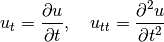
Many types of wave motion can be described mathematically by the equation 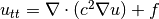 . We use a more compact notation for the partial derivatives to save space:
Let’s implement a solver for the 1D scalar acoustic wave equation with absorbing boundary conditions. Let  be the displacement at time t and at space location x, which is the wavefield. The displacement function
  is governed by the following mathematical model.
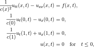
where the middle two equations are the absorbing boundary conditions, the last equation gives initial conditions, ![x \in [0,1]](_images/math/2ebe2a3059485f8f04d499a4c0c6baa8c17d0689.png) , and
, and ![t \in [0,T]](_images/math/6f68eb07534568e9d5d78042fcdebc89b95e1c2f.png) . The model velocity is given by the function
. The model velocity is given by the function  .
.
In our notation, we write that solving this PDE is equivalent to applying a nonlinear operator  to a model parameter
  , where
  for the scalar acoustics problem.
We then write that ![\mathcal{F}[m] = u](_images/math/e7a9acca63e1b9c0b6ffd5d7f34f5e4d1c4b4268.png) .
.
Contents: