1.1. Seismic Sources¶

$f(x,t)$ is the force function or source function in the above equation. We need to define it first.

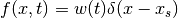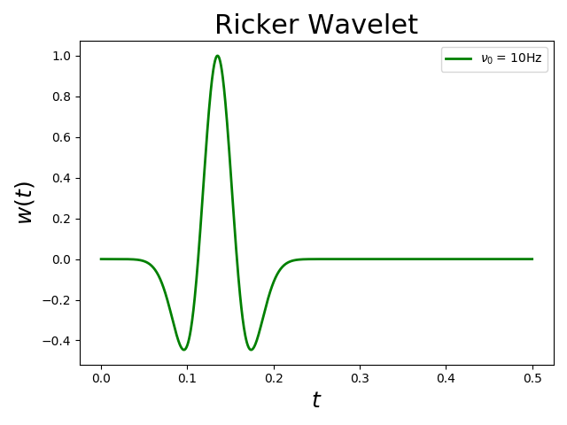
We define our source functions as $f(x,t) = w(t)\delta(x-x_s)$ , where $w(t)$ is the time profile, $\delta$ indicates that we will use point sources, and the source location is $x_0$ . In real world applications, the time profile is not known and is estimated as part of the inverse problem. However, it is common to model source signals with the negative second derivative of a Gaussian, also known as the Ricker Wavelet:

$w(t) = (1-2\pi^2\nu_0^2t^2)e^{-\pi^2\nu_0^2t^2}$

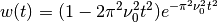
where $\nu_0$ is known as the characteristic or peak frequency (in Hz), because the magitude of $w$ ‘s Fourier transform $|\hat w|$ attains its maximum at that frequency. It is also important that this function is causal ( $w(t) = 0$ for $t\le 0$ ), so we introduce a time shift $t_0$ ,

$w(t) = (1-2\pi^2\nu_0^2(t-t_0)^2)e^{-\pi^2\nu_0^2(t-t_0)^2}.$

Problem 1.1

Write a Python function ricker(t, config) which implements the Ricker Wavelet, taking a time t in seconds and your configuration dictionary. This function should assume that your configuration dictionary has a key nu0 representing the peak frequency, in Hz. Your function should returns the value of the wavelet at time t.

You can guarantee causality by setting $t_0= 6\sigma$ for $\sigma = \tfrac{1}{\pi\nu_0\sqrt{2}}$ , the standard deviation of the underlying Gaussian. You may also want to implement an optional threshold to prevent excessively small numbers.

Plot your function for $t = 0, \dots, T=0.5$ at $\nu_0 = 10\textrm{Hz}$ and label the plot.

# In fwi.py

def ricker(t, config):

    nu0 = config['nu0']
    sigmaInv = math.pi * nu0 * np.sqrt(2)
    cut = 1.e-6
    t0 = 6. / sigmaInv
    tdel = t - t0
    expt = (math.pi * nu0 * tdel) ** 2
    w = np.zeros([t.size])
    w[:] = (1. - 2. * expt) * np.exp( -expt )
    w[np.where(abs(w) < 1e-7)] = 0

    return w

# Configure source wavelet
config['nu0'] = 10 #Hz

# Evaluate wavelet and plot it
ts = np.linspace(0, 0.5, 1000)
ws = ricker(ts, config)

plt.figure()
plt.plot(ts, ws,
         color='green',
         label=r'$\nu_0 =\,{0}$Hz'.format(config['nu0']),
         linewidth=2)
plt.xlabel(r'$t$', fontsize=18)
plt.ylabel(r'$w(t)$', fontsize=18)
plt.title('Ricker Wavelet', fontsize=22)
plt.legend();